Example 6 - Set Travel Time Target
In this example we will revisit the ANUGA model output we looked at in Example 1 - Particles in Steady Flow (ANUGA). This time, however, we will set a particle travel time target as opposed to a number of iterations for the particles to move.
In this method, we allow the particles to take as many iterations as they need (individually) to get as close as possible to the target travel time that we prescribe.
Full example script available here.
After loading the data and establishing the parameters in the same way we did in Example 1 - Particles in Steady Flow (ANUGA), we will change the grid size so that the range of travel times we can obtain in this small example is a bit better constrained. Then we will just define our particle seeding locations and generate the particles so they can be used for the routing.
>>> params.dx = 10.
# set up the particles
>>> seed_xloc = list(range(20, 30))
>>> seed_yloc = list(range(48, 53))
>>> Np_tracer = 50
>>> particle = pt.Particles(params)
>>> particle.generate_particles(Np_tracer, seed_xloc, seed_yloc)
We note that by discretizing our grid and the particle routing procedure, we are unable to prescribe precise particle travel times. Due to the gridded scheme, we can only measure particle travel times when particles are located at the center of a cell. So when a target travel time is set, the particle travel times are not precisely that number, but rather the closest times corresponding to when each particle is in a cell center.
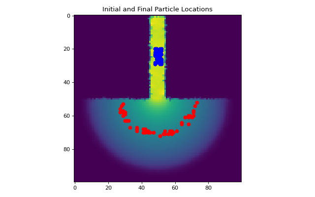
To set a travel time target, we will use the lower-level API and access the particle_track module directly, and then use some routines to plot the initial and final particle locations. The target travel time we will be using is 2100 seconds.
>>> walk_data = particle.run_iteration(target_time=2100)
>>> routines.plot_state(params.depth, walk_data, iteration=0, c='b')
>>> routines.plot_final(params.depth, walk_data, iteration=-1, c='r')
>>> plt.title('Initial and Final Particle Locations')
>>> plt.show()

To see how close we are to the prescribed target travel time of 2100 seconds, we will get a list of the final travel times that we then print to the console. We can access the data from the most recent step using get_state.
>>> _, _, finaltimes = routines.get_state(walk_data)
>>> print('List of particle travel times for final particle locations: ' +
>>>       str(np.round(finaltimes)))

List of particle travel times for final particle locations: [2042. 2064.
2106. 2087. 2085. 2102. 2069. 2089. 2090. 2091. 2051. 2106.
2111. 2119. 2140. 2129. 2101. 2083. 2091. 2145. 2179. 2080. 2067. 2100.
2163. 2096. 2125. 2079. 2129. 2151. 2122. 2089. 2137. 2112. 2093. 2093.
2102. 2102. 2099. 2042. 2070. 2108. 2115. 2115. 2108. 2112. 2062. 2124.]