Quickstart

Quick guide to using the dorado package using the 2 built-in sample datasets. The first demo provides an example of how to use the high-level API, while the second shows how functions can be accessed at a lower-level.

Demo 1- Using the High-Level API

In this demo, we show how particles can be routed along a simulated river delta, example output is from the delta simulation model, DeltaRCM. To do this, we will be using one of the high-level API functions provided in routines.py. A set of 50 particles will be seeded in the main channel of the synthetic delta. Then using information about the water depths and flow rates in the delta, the particles will be allowed to travel downstream. River deltas are distributary networks, and so the particles will not all travel along the same channels. By using a tool like dorado, simulated particles can help us answer questions related to hydrological connectivity and nutrient residence times in deltaic systems.

First we load and create the sample particles object.

>>> import dorado
>>> import matplotlib.pyplot as plt
>>> from dorado.example_data import define_params as dp
>>> rcmparticles = dp.make_rcm_particles()

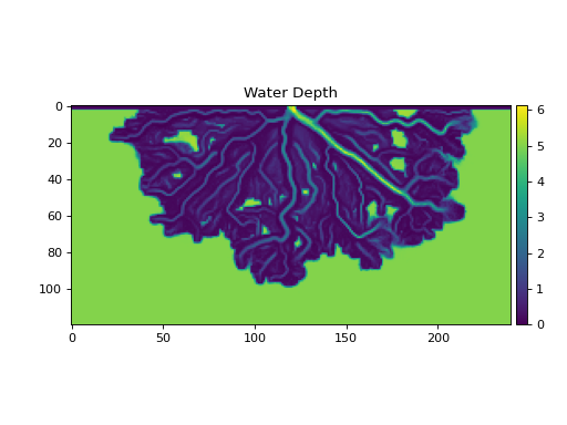
We can visualize the water depth for this scenario from the rcmparticles object. If you’d like to download this portion of the demo as a standalone script, it is available here.

>>> plt.imshow(rcmparticles.depth)
>>> plt.colorbar()
>>> plt.title('Water Depth')
>>> plt.show()

(png, hires.png)

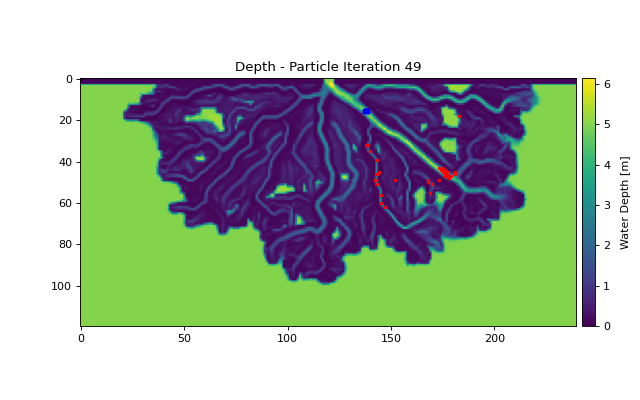
Now let’s route 50 particles for 50 iterations.

>>> dorado.routines.steady_plots(rcmparticles, 50, 'demo-1')

The steady_plots() function saves plots of each iteration of the particle movement to the subfolder ‘demo-1/figs’. The final plot is shown below; the initial particle locations are shown as blue dots, and the final particle locations are red dots. If you’d like to download this portion of the demo as a standalone script, it is available here.

(png, hires.png)

Demo 2 - Using Lower-Level Functionality

In this demo, we show how particles can be placed on a gridded flow field generated using the ANUGA software package. Instead of specifying the number of iterations for the particles to walk, we will be specifying a target travel time for the particles to travel in this demo. To do this, we will use some of the lower-level functionality accessible in particle_track.py.

First we load the grid parameters for this example. The longer Examples provide guidance on how to define your own grid parameters.

>>> import dorado
>>> import dorado.particle_track as pt
>>> from dorado.example_data import define_params as dp
>>> anugaparams = dp.make_anuga_params()

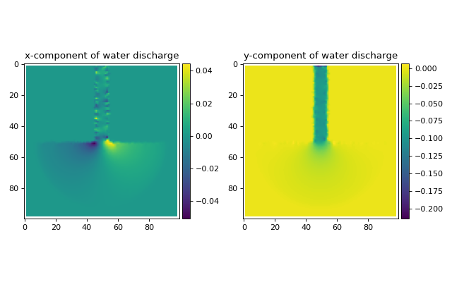
We can visualize the flow discharge components for this scenario from the loaded parameters. The full script used to produce the below figures is available here.

>>> plt.subplot(1, 2, 1)
>>> plt.imshow(anugaparams.qx)
>>> plt.title('x-component of water discharge')
>>> plt.subplot(1, 2, 2)
>>> plt.imshow(anugaparams.qy)
>>> plt.imshow(anugaparams.qy)
>>> plt.title('y-component of water discharge')
>>> plt.show()

(png, hires.png)

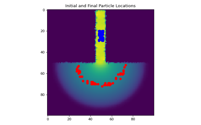
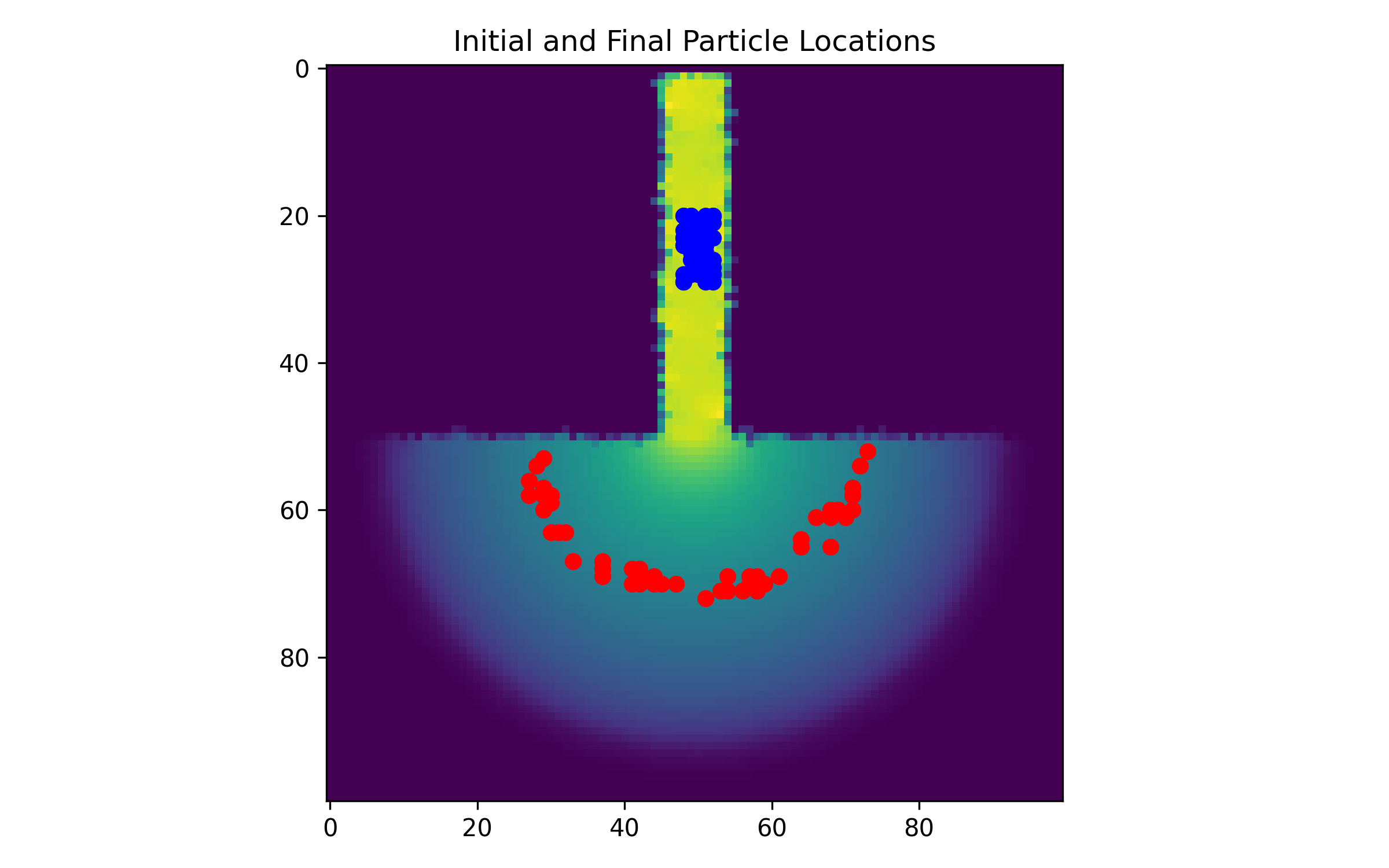
Now let’s route 50 particles with a target travel time of 2100 seconds. To do this, we first will need to define an instance of the dorado.particle_track.Particles class. Then we will generate a set of 50 particles to be routed. Finally we will actually move the particles until the target travel time of 2100 seconds is reached.

We will then visualize the final positions of the particles and display the final travel times associated with each of the particles to see how close they are to the target of 2100 seconds.

Note

The dorado method of routing particles in discrete grid cells limits the precision which can be achieved in travel time values as the particles can only be located at the center of grid cells.

The full script to produce the below figure and output is available here.

# initialize the particles class
>>> particles = pt.Particles(anugaparams)

# define where to place particles
>>> seed_xloc = list(range(20, 30))
>>> seed_yloc = list(range(48, 53))

# now generate particles and route them
>>> particles.generate_particles(50, seed_xloc, seed_yloc)
>>> walk_data = particles.run_iteration(target_time=2100)

# plotting
>>> dorado.routines.plot_state(particles.depth, walk_data, iteration=0, c='b')
>>> dorado.routines.plot_state(particles.depth, walk_data, iteration=-1, c='r')
>>> plt.title('Initial and Final Particle Locations')
>>> plt.show()

(png, hires.png)

>>> _, _, finaltimes = dorado.routines.get_state(walk_data)
>>> print('List of particle travel times for final particle locations: ' +
>>>       str(np.round(finaltimes)))

List of particle travel times for final particle locations: [2158.
2118. 2088. 2149. 2096. 2206. 2104. 2104. 2207. 2137. 2097. 2147.
2032. 2118. 2084. 2037. 2066. 2076. 2104. 2108. 2033. 2101. 2080.
2072. 2031. 2041. 2076. 2063. 2125. 2102. 2140. 2178. 2173. 2097.
2104. 2189. 2061. 2112. 2074. 2095. 2100. 2177. 2069. 2032. 2050.
2086. 2036. 2109. 2078. 2047.]